Plot Package

The up.plot package contains some high level methods to plot: * The plans * The variation of one or more (boolean or numeric) expression and quality metric values during a SequentialPlan * The causal graph of a Problem

Imports

Here are the imports needed for the following examples:

import unified_planning
from unified_planning.plans import (
    SequentialPlan,
    TimeTriggeredPlan,
    PartialOrderPlan,
    ContingentPlanNode,
    ContingentPlan,
    STNPlanNode,
    STNPlan,
)
from unified_planning.plot import (
    plot_plan,  # plot_plan plots all the types of plans, but is not customizable, while specific methods
    plot_sequential_plan,
    plot_time_triggered_plan,
    plot_partial_order_plan,
    plot_contingent_plan,
    plot_stn_plan,
    plot_causal_graph,
)

from unified_planning.model import (
    InstantaneousAction,
    DurativeAction,
    TimepointKind,
    Fluent,
    Problem,
    Object,
)
from unified_planning.shortcuts import (
    BoolType,
    UserType,
    IntType,
    RealType,
    TRUE,
    FALSE,
    Not,
)

SequentialPlan Example

A SequentialPlan is simply a sequence of actions.

actions = list((InstantaneousAction(f"a{i}") for i in range(1, 5)))
sequential_plan = SequentialPlan([a() for a in actions])

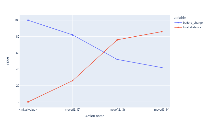
Plotting fluents in SequentialPlan

On a SequentialPlan, if the UPSequentialSimulator supports the Problem, the value of some arbitrary expressions or the value of some quality metrics can be plotted. This shows how the value changes during the plan.

Only numeric or boolean expressions can be plotted.

Define the problem:

The problem defined is a robot that moves from l1 to l4, passing through l2 and l3.

While moving, the battery decreases based on the distance from the locations and the total distance accumulates.

Note: the problem has specified only the parts interesting for this simulation. It’s not a complete problem to give to a planner.

Plot the value of the battery and the total distance during the plan simulation.

# Define the UserType
Location = UserType("Location")

# Define fluents
robot_at = Fluent("robot_at", BoolType(), position=Location)
battery_charge = Fluent("battery_charge", RealType(0, 100))
distance = Fluent("distance", IntType(), l_from=Location, l_to=Location)
total_distance = Fluent("total_distance", IntType())

# Define the move action
move = InstantaneousAction("move", l_from=Location, l_to=Location)
l_from = move.parameter("l_from")
l_to = move.parameter("l_to")
move.add_precondition(robot_at(l_from))
move.add_effect(robot_at(l_from), False)
move.add_effect(robot_at(l_to), True)
move.add_decrease_effect(battery_charge, distance(l_from, l_to) / 2 + 5)
move.add_increase_effect(total_distance, distance(l_from, l_to))

# Define the Location Objects
objects = list((Object(f"l{i}", Location) for i in range(1, 5)))
l1, l2, l3, l4 = objects

# Create the problem, add fluents, the move action and the objects
problem = Problem("moving robot")
problem.add_fluent(robot_at, default_initial_value=False)
problem.add_fluent(battery_charge, default_initial_value=100)
problem.add_fluent(distance, default_initial_value=0)
problem.add_fluent(total_distance, default_initial_value=0)
problem.add_action(move)
problem.add_objects(objects)

# Set the initial values different from the defaults
problem.set_initial_value(robot_at(l1), True)
problem.set_initial_value(distance(l1, l2), 26)
problem.set_initial_value(distance(l2, l3), 50)
problem.set_initial_value(distance(l3, l4), 10)

# Create the plan to simulate
plan = SequentialPlan(
    [
        move(l1, l2),
        move(l2, l3),
        move(l3, l4),
    ]
)

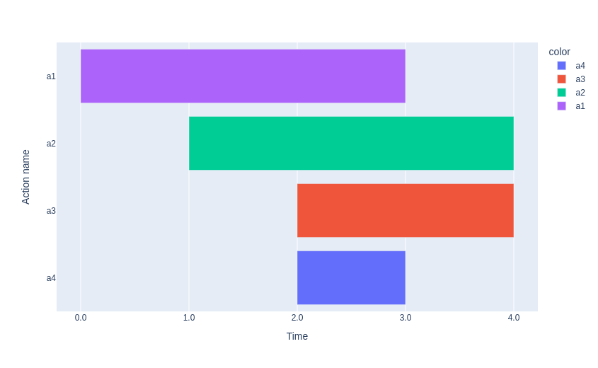
_images/sequential_plan_fluents_plot.png

TimeTriggeredPlan Example

A TimeTriggeredPlan is a sequence of 3 items. Every items is composed by an action, the time in which the action starts, and, if the action is a DurativeAction, the action duration.

a1, a2, a3, a4 = (DurativeAction(f"a{i}") for i in range(1, 5))
time_triggered_plan = TimeTriggeredPlan(
    [
        (0, a1(), 3),
        (1, a2(), 3),
        (2, a3(), 2),
        (2, a4(), 1),
    ]
)

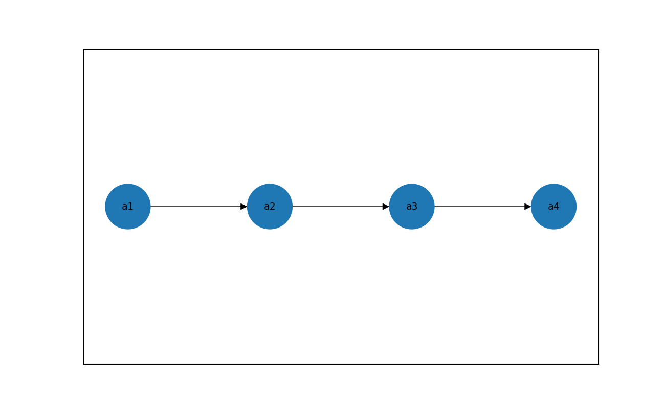
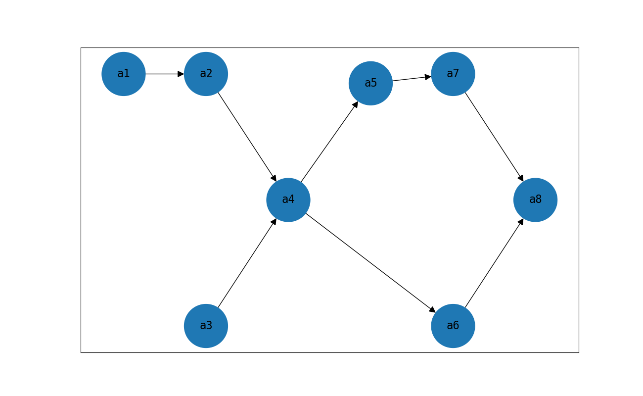
Partial Order Plan

A PartialOrderPlan is a directed graph where the nodes are ActionInstances and the edges create an ordering between 2 actions.

In the unified_planning, a PartialOrderPlan is created with the adjacency list.

Generally speaking, a SequentialPlan is a specific case of a PartialOrderPlan where every action has only one possible action that must be done before and one action that must be done later.

ai1, ai2, ai3, ai4, ai5, ai6, ai7, ai8 = (
    InstantaneousAction(f"a{i}")() for i in range(1, 9)
)
partial_order_plan = PartialOrderPlan(
    {
        ai1: [ai2],
        ai2: [ai4],
        ai3: [ai4],
        ai4: [ai5, ai6],
        ai5: [ai7],
        ai6: [ai8],
        ai7: [ai8],
    }
)

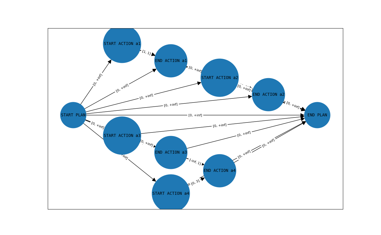
STNPlan Example

An STNPlan represents the temporal constraints from the events that must be performed during the plan.

An event is either the start of the plan, the end of the plan, the start of an action or the end of an action.

It is represented as a directed graph, where the nodes are the events.

There is an edge from the node N to the node M if N and M have a relative temporal constraint. The edge is labeled with 2 numbers, the lower bound and the upper bound to the time that can elapse from N to M.

For example: N –[0, 7]–> M means that M must happen after -or at the same time, since 0 is included- N, but no more than 7 time units later.

ai1, ai2, ai3, ai4 = (InstantaneousAction(f"a{i}")() for i in range(1, 5))
start_a1 = STNPlanNode(TimepointKind.START, ai1)
end_a1 = STNPlanNode(TimepointKind.END, ai1)
start_a2 = STNPlanNode(TimepointKind.START, ai2)
end_a2 = STNPlanNode(TimepointKind.END, ai2)
start_a3 = STNPlanNode(TimepointKind.START, ai3)
end_a3 = STNPlanNode(TimepointKind.END, ai3)
start_a4 = STNPlanNode(TimepointKind.START, ai4)
end_a4 = STNPlanNode(TimepointKind.END, ai4)
stn_plan = STNPlan(
    [
        (start_a1, 1, 1, end_a1),  # Link start to end actions
        (start_a2, 0, 3, end_a2),
        (start_a3, 0, 3, end_a3),
        (start_a4, 0, 3, end_a4),
        (
            end_a1,
            0,
            None,
            start_a2,
        ),  # Action 1 must finish before action 2 start (or in the same moment)
        (
            end_a3,
            None,
            1,
            end_a4,
        ),  # Action 3 can finish AT most 1 after the end of Action4
    ]
)

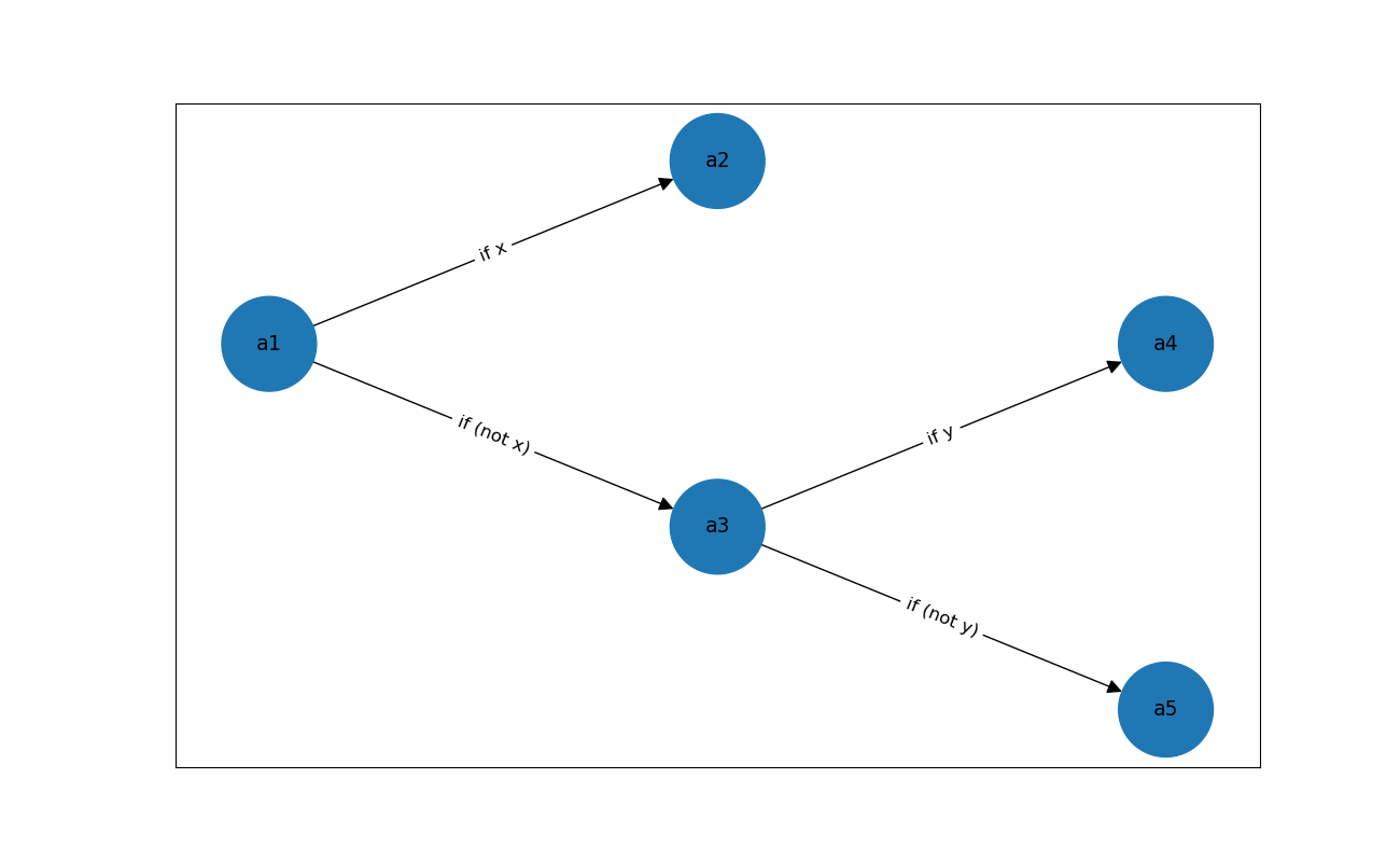
Contingent plan Example

A ContingentPlan is represented as a decision tree. Some actions can sense the initially unknown value of one or more fluents and decide which action to perform next based on the sensed values.

It is represented as a directed graph, with the nodes containing the action to perform and the edges labeled as the expression that must be True in order to take that branch.

ai1, ai2, ai3, ai4, ai5 = (InstantaneousAction(f"a{i}")() for i in range(1, 6))
node_1 = ContingentPlanNode(ai1)
node_2 = ContingentPlanNode(ai2)
node_3 = ContingentPlanNode(ai3)
node_4 = ContingentPlanNode(ai4)
node_5 = ContingentPlanNode(ai5)
x, y = Fluent("x"), Fluent("y")
node_1.add_child({x(): TRUE()}, node_2)
node_1.add_child({x(): FALSE()}, node_3)
node_3.add_child({y(): TRUE()}, node_4)
node_3.add_child({y(): FALSE()}, node_5)
contingent_plan = ContingentPlan(node_1)

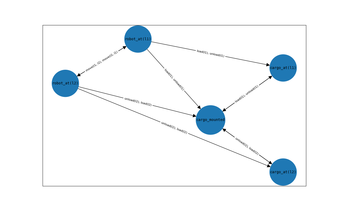
Causal Graph

The causal graph of a problem shows how the different (grounded) fluents of the problem are interwined by the actions.

Every node of the graph is a fluent and there is an arc from F1 to F2 if there is an action in the problem that reads F1 and writes F2. If an action writes both F1 and F2 the arc from F1 to F2 will be bidirectional.

The edge labels are the actions that use both fluents.

Define the problem:

The problem has a cargo at Location l2 that must be moved by a robot to a Location l1.

# Define UserTypes
Location = UserType("Location")

# Define Fluents
robot_at = Fluent("robot_at", BoolType(), position=Location)
cargo_at = Fluent("cargo_at", BoolType(), position=Location)
cargo_mounted = Fluent("cargo_mounted")

# Define move action
move = InstantaneousAction("move", l_from=Location, l_to=Location)
l_from = move.parameter("l_from")
l_to = move.parameter("l_to")
move.add_precondition(robot_at(l_from))
move.add_precondition(Not(robot_at(l_to)))
move.add_effect(robot_at(l_from), False)
move.add_effect(robot_at(l_to), True)

# Define load action
load = InstantaneousAction("load", loc=Location)
loc = load.parameter("loc")
load.add_precondition(cargo_at(loc))
load.add_precondition(robot_at(loc))
load.add_effect(cargo_at(loc), False)
load.add_effect(cargo_mounted, True)

# Define unload action
unload = InstantaneousAction("unload", loc=Location)
loc = unload.parameter("loc")
unload.add_precondition(robot_at(loc))
unload.add_precondition(cargo_mounted)
unload.add_effect(cargo_at(loc), True)
unload.add_effect(cargo_mounted, False)

# Define objects
l1 = Object("l1", Location)
l2 = Object("l2", Location)

# Create the problem and add fluents, actions and objects
problem = Problem("robot_loader")
problem.add_fluent(robot_at, default_initial_value=False)
problem.add_fluent(cargo_at, default_initial_value=False)
problem.add_fluent(cargo_mounted, default_initial_value=False)
problem.add_action(move)
problem.add_action(load)
problem.add_action(unload)
problem.add_objects((l1, l2))

# Set initial value and goals
problem.set_initial_value(robot_at(l1), True)
problem.set_initial_value(cargo_at(l2), True)
problem.add_goal(cargo_at(l1))

# Plot the causal graph